Author: Karunakar Gumudala
Introduction:
Spatial datasets always are more than a few gigabytes in size, with millions of records each. And naturally, when it comes to processing them, it can be a herculean task. Spatial datasets are geo files that can be parsed and processed best by geoprocessing modules of Python such as pandas, numpy, shapely, GeoPandas. This article discusses the effectiveness of the Python geopanda package in analyzing geo calculations like the distance between geo locations (latitudes and longitudes), finding the existence of a geolocation in a geo area, etc. In order to process millions of records, one would need to make use of parallel processing modules like joblib, dask, etc. In addition to that, Geopandas have spatial joins which are very efficient in processing thousands of records in just a few seconds.
Problem Statement:
Ideally, owners of homes will want to admit their children only into those schools into whose boundaries their homes fall. Several homes can fall into a region/boundary of a school and a single home can fall into multiple school boundaries. In order to find out which school a child must go to, let us consider two datasets – Dataset 1 that has details of the homes, and Dataset 2 that has details of the schools.
Dataset 1:
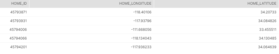
This dataset consists of geolocations of homes in the USA. Each home is represented by a longitude and a latitude. Generally, longitude values range from -180 to 180, and latitude values range from -90 to 90 (in degrees).
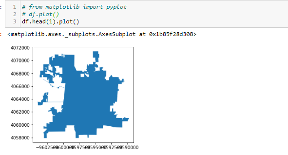
The below image consists of a few examples of geolocations of homes in the US-
Dataset 2:
This dataset consists of geo regions of all the schools present in all the states in the US. A geo region represents the boundary of a school.
The datasets can be downloaded from https://nces.ed.gov/programs/edge/SABS (user .shp file)
Challenges:
1. The number of homes was around 100 million and the number of school boundaries was around 75 thousand.
2. We are using Snowflake Warehouse for our data analysis. Snowflake does not support reading .shp files directly. It has the spatial function “haversine distance” to find the distance between two geolocations. SQL Server and Postgresql have spatial functions, but analyzing such large volumes of data on RDS (Relational Database System) is not recommended.
3. And of course, the age-old problem of finding a solution with minimal use of resources and time.
Solution Approach:
For this particular problem, the GeoPandas Python library is the perfect fit. The goal of GeoPandas is to make working with geospatial data in Python easier. It combines the capabilities of pandas and shapely, providing geospatial operations in pandas and a high-level interface to multiple geometries to shapely. GeoPandas enables to easily accomplish operations in python that would otherwise require a spatial database such as PostGIS.
Step 1:
The geo-datasets downloaded here are then read using the GeoPandas library in Python.
Once the data is read, we create two geodataframes – one from the homes dataset and another from the dataset containing the school boundaries.
Geodataframe for homes: A home is represented by geo-coordinates i.e., longitude and latitude. First, the homes with their coordinates should be brought into a pandas dataframe. Then we create a geoPandas data frame as follows.
Creation of pandas data frame:
import pandas
input_geopoints = pandas.read_csv(csvfile with Longitude and Latitude columns)
Creation of geo data frame from pandas data frame:
import geopandas
geopoints = geopandas. GeoDataFrame(input_geopoints,geometry=geopandas.points_from_xy(input_geopoints.Longitude,input_geopoints.Latitude))
where input_geopoints is a pandas dataframe with longitude and latitude, and geopoints is a geo dataframe.
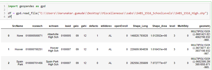
Geodataframe for School Boundaries: Geo regions come with the .shp extension and are called shapefiles.
Create geo dataframe from shape files
georegions =geopandas.read_file(shapefile.shp)
where shapefile.shp is a shape file and georegions is a geodataframe
Let us call these two dataframes geopoints and georegions.
Note : The two geodataframes must have the same SRId (Spatial Reference Id). A typical SRId would be 4326. SRId 4326 refers to spatial data that uses longitude and latitude coordinates on the Earth’s surface as defined in the WGS84 standard, which is also used for the Global Positioning System. We can ensure that both the data frames have the same SRId by using the commands, geopoints.crs and georegions.crs. If they are not the same, we can change it to common SrId by-
geopoints.crs = {‘init’: ‘epsg:4326’}
georegions.crs = {‘init’: ‘epsg:4326’}
To understand more about spatial referencing, visit https://spatialreference.org/
Step 2:
Once the dataframes are ready, we need to process them, i.e., extract the pairs of “points and regions” where a point falls into regions. To do this, geopandas has joins called spatial joins. Spatial joins are the joins that can be performed on geodataframes. The dataframes are combined based on the spatial relationship to one another.
For example, let us consider two dataframes-
gdf1 – dataframe with longitude and latitude
gdf2 – dataframe with shapes
Now, we can combine these datasets with spatial join as below-
geopandas.sjoin(gdf1,gdf2,op=”within”)
which means to create a dataframe based on whether a geopoint falls into a shape or not.
The following statement is used to perform the join
geopandas.sjoin(geopoints,georegions)
This results in a pandas dataframe with the points and all the shapes into which the points fall into.
The performance can be improved by creating spatial indices before doing the above join using the commands geopoints.sindex and georegions.sindex.
Spatial indices significantly boost the performance of the spatial queries. These are based on the R-Tree data structure. The core idea behind the R-tree is to form a tree-like data structure where nearby objects are grouped together, and their geographical extent(minimum bounding box) is inserted into the data structure. This bounding box then represents the whole group of geometries as one level (typically called “page” or “node”) in the data structure. This process is repeated several times, which produces a tree-like structure where different levels are connected to each other. This structure makes the query times for finding a single object from the data much faster, as the algorithm does not need to travel through all geometries in the data.
We did some research and realized no optimization other than the above is required, as geopandas spatial joins internally makes use of advanced data structures like R-trees.
Note: In this particular case, the number of homes (geopoints rows) was around 140 million and the number of georegions was around 75 thousand. Because of this, each home had to be processed against 75 thousand regions and as a whole, 140 million homes had to be processed against 75000 regions. Obviously, processing the two datasets in one go is not at all a good idea.
And so, we shall split the homes into a certain number of batches and then process them against the regions. The following points have to be considered in such a scenario-
1. The size of a batch, i.e., how many homes should be considered in one go?
2. Should the batches be processed sequentially or in parallel?
To answer the above two questions, we must look into the size of resources (memory and core) that is available at one’s disposal.
For this study, we implemented sequential processing. With 4 core and 8GB machine, for batches of 10k, it took about 4–5 seconds for each batch process. Hence all 140 million geopoints were processed in about 20 hours. Alternatively, if time is of concern, then one can opt for parallel processing. The dask (https://dask.org/) module in Python can be used for parallel processing.
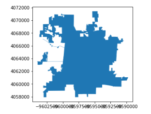
Conclusion:
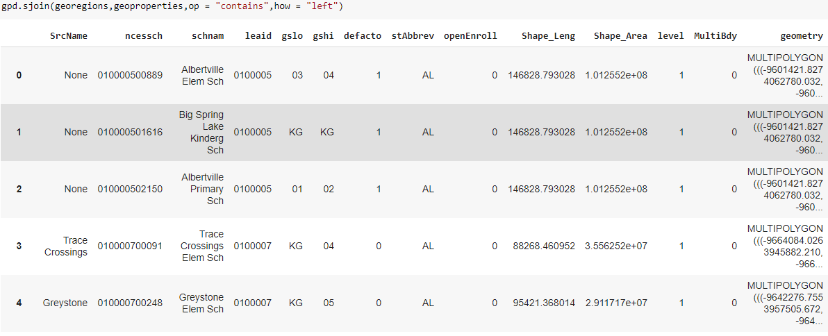
The below image shows a snapshot of the results of this exercise-
Using geopandas to process spatial datasets saves a lot of time, and also gives an option of not having to invest in proprietary GIS software and tools. The complete working notebook is available over here – https://colab.research.google.com/drive/1UKHoG5I5OqSXbRBd0PTGPVB3162GTyve?usp=sharing
Further learning:
1. To reduce the processing time, we can try multiprocessing on the above batches. Warning: Multiprocessing is CPU intensive.
2. There are two other Python libraries (numba and dask) that can help us further improve the performance of the processing.
3. There are also third party spatial APIs available to help with geoprocessing- https://datasystemslab.github.io/GeoSpark/download/overview/