It is 1892. Sherlock Holmes stands in a moonlit stable where a prized racehorse has vanished. The decisive clue is not something that happened, it is something that did not. The dog made no sound. Silence, correctly interpreted, revealed the truth.
Retail pricing systems face the same challenge. A product records two consecutive weeks of slowing sales. The discounting engine recommends a deeper markdown. Days later, the team discovers that the top-selling sizes had been out of stock for much of that period. Sales declined not because demand weakened, but because inventory was unavailable.
Discounting reacts quickly. Context surfaces later. By the time the full picture emerges, the margin has already absorbed the impact.
The real issue is not whether a product is selling. It is whether the system has accurately interpreted what the sales data represents, and whether the decision to discount was grounded in demand reality or operational noise.
Two Systems, One Difference that Changes Everything
The original discounting framework operated at a category level. Products were ranked against peers, and markdowns were triggered by relative sell-through within defined calendar windows. Consistent, but structurally limited.
The redesigned framework evaluates each product group against its own expected seasonal trajectory, not against how peers are performing this week. That single shift, from peer comparison to self-comparison across time, changes every downstream decision.
Is this product selling the way it should be selling, at this specific point in its own season?
That question, answered with structure, is the foundation of demand discipline.
The Structural Limits of Outcome-Based Discounting
Most discounting engines react to observed results: slow sales trigger markdowns, strong sales validate pricing, late-season inventory triggers escalation. The execution is consistent. The problem is that sales data does not automatically isolate consumer demand, it reflects timing, availability, size-level breakage, and replenishment gaps all at once. Four structural gaps tend to follow:
- Products evaluated against peers, not their own seasonal pace, so an on-track product can trigger a markdown simply because a peer outperformed it this week.
- Broad discounting windows that apply to on-track items alongside genuine underperformers.
- Inventory pressure that only becomes visible after it has accumulated, forcing compressed late-season correction.
- Temporary availability gaps that reduce observed sales without reducing underlying demand, and the system cannot tell the difference.
Together these gaps create premature discounting, late escalation, and margin erosion that is hard to reverse mid-season. The fix requires a different starting question:
Is the gap a demand problem, or something else entirely?
Answering that reliably requires a seasonal baseline: a defined expectation of how demand should accumulate over time. Without it, routine volatility triggers unnecessary intervention. With it, performance can be evaluated against expected pace rather than short-term noise, and in seasonal retail, that distinction separates preserved margin from eroded margin.
A Specialty Apparel Retailer: Why Timing is Everything
We collaborated with a leading American speciality apparel retailer operating within tightly defined seasonal cycles. Inventory commitments were finalised ahead of peak periods, and unsold stock carried forward to the next season, accruing holding costs while occupying capital that could have been redeployed.
A markdown applied two weeks too early surrendered margin on items that would have sold at full price. Two weeks too late required deeper discounting to clear stock before the window closed. The retailer’s rule-based system was consistent but exhibited every structural gap described above. The framework we developed was built to close them, not by replacing human judgment, but by giving that judgment a more reliable signal.
Seasonal Pacing as the Discounting Baseline
The foundation of the redesigned framework is the Expectation Sales Curve: a week-by-week model of how demand accumulates across a season, built from multiple years of historical full-price data. Rather than working with raw volumes, sales are converted into cumulative percentage-of-season contributions, making the model about timing, not scale.
If historical data shows that 35% of seasonal sales typically occur by week six, then week six performance should align with that benchmark. If cumulative sales reflect what is typical of week four, the product is not simply slow, it is two weeks behind its expected pace.
That distinction determines urgency and shapes the intervention. The curve does not set sales targets. It defines expected accumulation patterns, the reference baseline against which every downstream metric is measured.
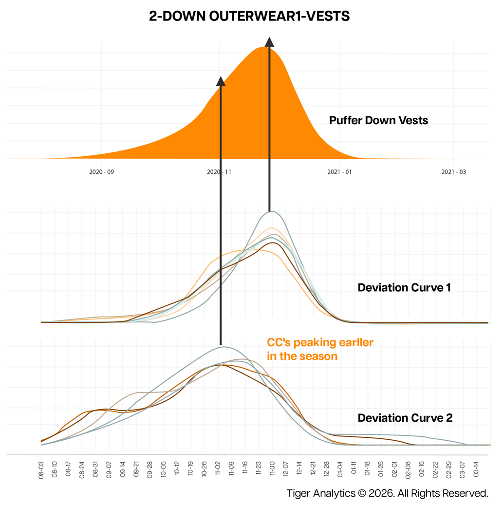
How demand trajectories diverge from the expected seasonal curve, products peaking earlier signal early deviation.
The Metrics that Translate Trajectory into Decisions
Three core metrics convert expected trajectory into operational signals.
1. Sale Lag and Sale Lag Ratio
Sale Lag measures deviation from the Expectation Sales Curve in time units. If a product’s cumulative performance aligns with where the curve predicted two weeks earlier, the product carries a two-week lag. Expressing deviation in weeks, rather than percentage, makes gaps immediately interpretable and anchors conversations to pace rather than contested figures.
The Sale Lag Ratio adjusts that lag against the remaining selling window. A two-week gap with twelve weeks of season left is a monitoring situation. The same gap with three weeks remaining requires immediate action. The ratio calibrates urgency as the runway shortens.
2. Accumulation Index
The Accumulation Index compares remaining on-hand inventory against expected remaining sell-through. When it rises, inventory is accumulating faster than demand is absorbing it, surfacing pressure before it becomes a late-season crisis and enabling measured correction rather than margin-damaging escalation.
3. Deviation Curve
Not every deviation reflects weakening demand. Size-level breakage, replenishment delays, and availability gaps all reduce observed sales without touching underlying demand. The Deviation Curve evaluates whether a deviation falls outside normal expected variance. Only confirmed demand gaps, after operational factors have been screened, progress to a discount decision.
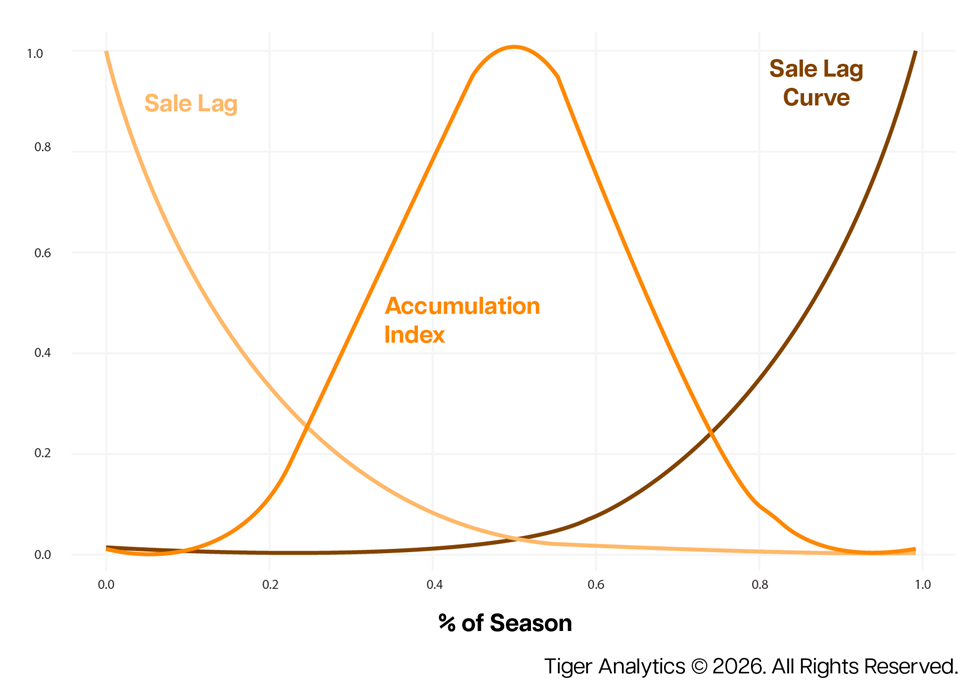
Sale Lag, Accumulation Index, and Sale Lag Curve plotted across the season, showing how inventory exposure and timing risk evolve.
The Weekly Decision Cadence
The framework runs on a structured weekly cadence at the product group level, evaluating each signal in deliberate sequence: trajectory gap, time lag, inventory exposure, deviation validation, delivery constraints, and discount-response estimates. The order matters, the system establishes context before measuring deviation and validates signals before considering intervention.
Shared dashboards surface time lags, inventory runway risk, recommended discount tiers, and projected velocity impacts, aligning merchandising, planning, and analytics teams around the same weekly signals. The cadence was reinforced through iterative simulation testing, embedding governance into the team’s standard commercial rhythm rather than treating it as a separate analytical exercise.
What Changed, and Why it Matters
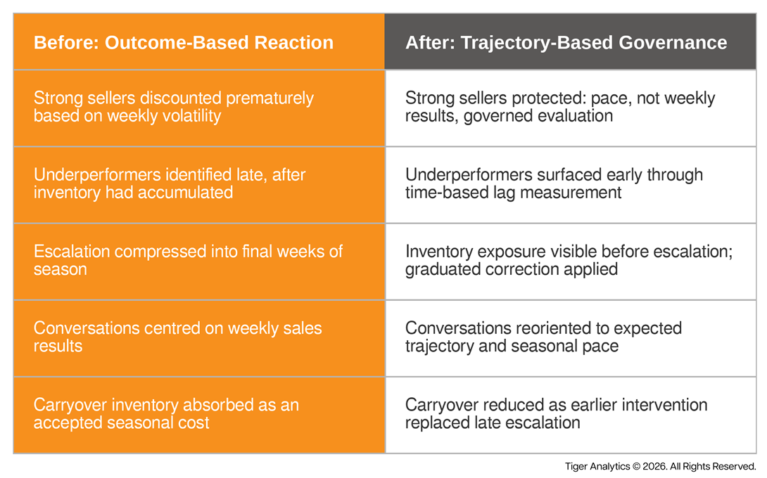
The less visible shift was in how teams asked questions. The weekly review moved from the retrospective; how did we do? to:
Are we on pace? And if not, is the gap a demand problem or something we can resolve without touching price?
Why Demand Discipline Creates a Competitive Advantage
When these disciplines are embedded in a weekly cadence, discounting stops chasing noise and begins managing timing. Retailers who build this capability compound the advantage across every season: less premature discounting, earlier course correction, lower carryover, and cross-functional conversations grounded in shared signals rather than competing interpretations of the same weekly report.
Structured interpretation defines timing. Timing defines margin. That is where demand discipline becomes a competitive advantage.